Fig.
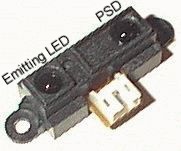
1 - Sharp GP2D12 distance sensor
Fig.
2- Sharp GP2D12 output pattern
Sharp GP2D12
Application note for an infrared, triangultation-based distance sensor with an analog, non-linear output
This application note is intended to provide a good overview of the Sharp GP2D12 sensor (Fig. 1) and its use, especially for dynamics application. I hope it will help some robotists to make this sensor work quite easily and to avoid certain pitfalls. This range finder is one of the most commonly used in autonomous robotics applications for hobbyists and also in academic research. The reasons for this are essentially its low price (about 14$ at Acroname, for example), its compact (~40x14x13mm) and lightweight package (a comparison between several sensors may be found here). The GP2D12 is based on the triangulation principle with a collimated infrared LED for the emitting element and a PSD (Position Sensing Device) which constitutes the receiver.
|
|
|
|
|
Fig.
1 - Sharp GP2D12 distance sensor
|
Fig.
2- Sharp GP2D12 output pattern
|
Although it exists a very similar sensor with a digital output (the GP2D02), I will focus only on the GP2D12 which has an analog output (see Fig. 2). The main motivation for this choice is that the digital version is almost twice slower than the GP2D12 (update period about 75ms against 40ms for the analog version). Table 1 gives a brief overview of the GP2D12 specifications.
|
Range:
|
10
to 80cm
|
|
|
Update
frequency / period:
|
25Hz / 40ms
|
|
|
Direction
of the measured distance:
|
Very directional,
due to the IR LED
|
|
|
Max
admissible angle on flat surface:
|
>
40°
|
|
|
Power
supply voltage:
|
4.5
to 5.5V
|
|
|
Noise
on the analog output:
|
<
200mV
|
|
|
Mean
consumption:
|
35mA
|
|
|
Peak
consumption:
|
about 200mA
|
|
|
Table
1 - Overview of the Sharp GP2D12 specifications
|
||
Note: it is very important to put a good capacitor (something like 22uF) between GND and Vcc, directly on the sensor itself, in order to reduce the noise on the 5V power supply due to the current required by the emitting LED. In the other hand, avoid the use of a capacitor between the signal output and GND or Vcc: it may dramatically reduce the sensor dynamics (low pass filter). Below, we will see how to numerically filter this output in order to improve the precision without decreasing the dynamics.
When powered with a 5V potential, the Sharp sensor has a maximum output voltage of about 2.45V, for close distances. The highest useable distance gives approximately 0.45V (see Fig. 2). It is therefore wise to use an AD converter with two external adjustable voltage references: Vref and COM (the one I employed is the MAX148BCAP). In order to obtain the best precision, the highest limit of the converter (255 on 8 bits) should more or less correspond to the highest output voltage of the sensor, that is the lowest measurable distance, and vice versa. In doing so, the full scale of the converter is used. Fig. 3 shows the measured result.
Fig. 3 - GP2D12 output pattern after AD conversion ( 0 ->
~0.45V & 250 -> ~2.45V )
Based on these measurements, a lookup table can be implemented in a microcontroller. For my own application, I used a Ubicom SX52 microcontroller with a 256 entries lookup table.
In order to measure the noise present on the sensor output, I made some tests and statistics with a GP2D12 sensor placed at about 25cm in front of a flat white wall. The distribution of 10'000 successive values acquired by the microcontroller (at 1kHz) is shown on Fig. 4.
Fig. 4 - Statistical analysis of the Sharp GP2D12 output
The values presented here are characteristic of the GP2D12 output. In particular, the standard deviation does not depend on the measured distance. However, the precision of the distance cannot be directly deduced because the output is non linear. A constant standard deviation over the full range of the sensor output does not lead to a constant precision of the computed distance.
This graph (Fig. 4) shows that the noise of the Sharp sensor output follows a normal-like distribution law. Therefore, it would be wise to average several successive output values to improve the precision.
Note that this quite important noise is essentially due to the sensor itself (electronic noise). The noise introduced by the converter is marginal. See Fig. 8 bellow to convince yourself.
As the employed 8-bit micro controller is not able to efficiently handle multiplications and divisions, a lookup table preferable to convert the output values of the sensors into distances (another approach, using a power regression, is explained here). As the converted values from the AD converter are 8-bit coded, the best we can do is to use a lookup table with 256 entries. The microcontroller offers the possibility to store 12-bit data in the program memory. It is therefore easy to store the distances in millimeters (from 100 to 800) that would require 10 bits.
As the microcontroller has not a lot of program memory, in the case of the use of several GP2D12, it seems wise to have a single table for all the sensors. The following graph (Fig. 5) shows the measured output patterns of 4 different sensors red simultaneously and several times at the same distance (only the average for each distances and each sensors are shown).
Fig. 5 - Characteristics of four different Sharp GP2D12 sensors
40 reference distances for each sensor have been defined in order to plot these graphs. A linear approximation between each pair of successive points is made. On the following graph (Fig. 6), only the actually measured points (for one of the four sensors) and their corresponding standard deviation are shown.
Fig. 6 - Set of 40 measured values and their corresponding standard deviation
Based on this graph, a rapid evaluation of the precision can be done. It is easy to understand that the values above 700mm are almost unusable. At 600mm, the precision is only 20mm and becomes better with closer distance (about 2mm at 200mm). Of course, using a unique lookup table for several sensors slightly decreases the precision, but however must represent a good compromise in certain cases.
The analog output of the Sharp GP2D12 sensors moves in voltage steps when the measured distance changes. These steps last about 40ms (see Fig. 7).
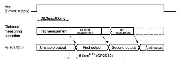
Fig. 7 - Sharp GP2D12 operation over time
This behavior is certainly due to the fact that it processes an output signal by internally averaging successive values. Let's assume that the best way to interpret this signal is to take the step level as the value measured at its middle. Because there is some noise on the sensor output, we can get an improved value of the distance by averaging the output along the step.
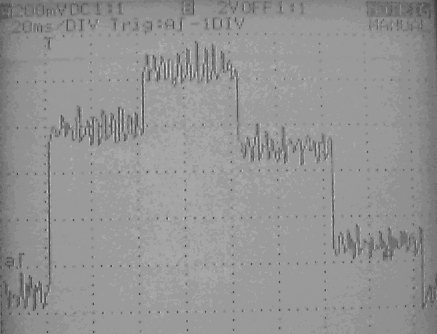
Fig. 8 shows the typical sensor output during a fast movement of the target object. As you can see, the noise on the steps can reach about ±100 mV.
Fig. 8 - Sharp sensor output during dynamic measurement (200mV and 20ms per division)
What is more interesting for us is the same signal seen by the microcontroller (Fig. 9).
Fig. 9 - Sharp sensor output seen by the microcontroller during dynamic measurement
The reading frequency of the converter is 1kHz. Therefore the processor can have an updated value every 1ms and thus about 40 values per step. These 40 values will be averaged over time in order to obtain a good approximation of the step level without noise (this procedure acts like a digital low-pass filter). To achieve this, the points belonging to the same steps must be recognized and clustered.
There are essentially two criteria to achieve this clustering. The first is certainly the difference between successive data. If the difference is greater than a specified threshold, the processor can know that it is the next step. The second one is the maximum time allowable for a step. If two of them are merged, we can end the set of successive values belonging to the same step by knowing the maximum length of this set. The maximum number of conversion during a step is 43. So if there is no significant transition after 43 readings, we can assume that future data are part of the next step. If some data are not well classified, in this case, this is not so important because it will not significantly change the mean value of the steps.
If all the steps are at the same height (static case), this clustering process will lose the synchronization. But, as soon as a transition appears, the algorithm will automatically synchronize again.
This algorithm has been implemented in the microcontroller. The computed means of the steps are represented in black on Fig. 10. Please note that the clustering is applied to the rough sensor values and not to the distances after conversion through the lookup table. This algorithm is intended to filter the noise of the sensor output, which is constant over the full scale of distances. If the successive values from the sensor were first converted into distances, the noise would have not always the same magnitude.
Fig. 10 - Result of the clustering processThe threshold for the difference is set to 15 and the maximum number of points belonging to the same step was 43.
We can see that there was not enough difference between the fourth and the fifth steps. Therefore the 43 first points have been allocated to the fourth step. And the last points (actually 38) before the next recognized transition are part of the fifth step.
Note that the computation of this average does not require 40 or 43 registers in memory. A sum variable on 16-bit is updated at each reading of the converter. When the end of a cluster is detected, the sum is divided by the number of data in the set. Each computed average will be then transformed into a distance via the lookup table. This distance is time stamped with the middle of the previous step.
To sum up, we have now an algorithm, which is able to process the rough sensor data at 1kHz and output an enhanced distance value about each 40ms i.e. at a frequency of 25Hz, which is the update rate of the Sharp GP2D12.
On the following graph (Fig. 11), the whole process is revealed through real values coming from the microcontroller in real time.
Fig. 11 - Clustering process and resulting distances
A point represents each acquired sensor value, every millisecond. The vertical gray lines indicate the moment when the end of a step has been detected: a jump higher than the specified threshold or the overrun of the maximum successive values allowable for one step. The little circles symbolize the distances at the moment they are calculated. The crosses are the same values but plotted at the position they are time stamped thus 60ms before their calculation.
Now, if several sensors are used, there will be several such processes, asynchronously. If simultaneous distances must be estimated (that was the case in my project), it is possible to implement a routine based on the above-described algorithm (see this document for further information).
Published: 22.03.01 Last update: 18.11.04 (29.04.01)